Interpretability
FF06 · ©2017 Cloudera, Inc. All rights reserved

This is an applied research report by Cloudera Fast Forward Labs. Originially released to subscribers in August 2017, it is now open to the public. We write reports about emerging technologies. Accompanying each report are working prototypes that exhibit the capabilities of the algorithm and offer detailed technical advice on its practical application. Read our full report on interpretability below or download the PDF. For this report we built an interpretability prototype: Refractor.
Introduction
Our society is increasingly dependent on intelligent machines. Algorithms govern everything from which e-mails reach our inboxes to whether we are approved for credit to whom we get the opportunity to date – and their impact on our experience of the world is growing.
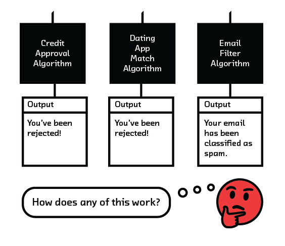
This rise in the use of algorithms coincides with a surge in the capabilities of black-box techniques, or algorithms whose inner workings cannot easily be explained. The question of interpretability has been important in applied machine learning for many years, but as black-box techniques like deep learning grow in popularity, it’s becoming an urgent concern. These techniques offer breakthrough capabilities in analyzing and even generating rich media and text data. These systems are so effective in part because they abstract out the need for manual feature engineering. This allows for automated systems that are able to do completely new things, but are unable to easily explain how they do those things.
Interpretability is relevant to anyone who designs systems using machine learning, from engineers and data scientists to business leaders and executives who are considering new product opportunities. It allows you to better understand your machine learning systems and thus generate more useful results. It helps to explain algorithmic predictions and therefore change real-world outcomes. It is necessary in regulated industries where you have to prove that business practices are not dangerous or discriminatory. Further, interpretability is a key tool in understanding bias and accountability in the increasingly automated systems we are deploying throughout society.
In this report, we explore two areas of progress in interpretability: systems designed to be perfectly interpretable, or white-box algorithms, and emerging research on approaches for inspecting black-box algorithms.
The Power of Interpretability
If a model makes correct decisions, should we care how they are made? More often than not, the answer is a resounding yes. This chapter explains why.
What Is Interpretability?
From the point of view of a business deploying machine learning in a process or product, there are three important kinds of interpretability:
- Global – Do you understand the model as a whole to the extent required to trust it (or to convince someone else that it can be trusted)?
- Local – Can you explain the reason for a particular decision?
- Proxy – When the model is a perfect proxy for the system you are interested in, can you say how the model works, and thus learn about how the real system works?
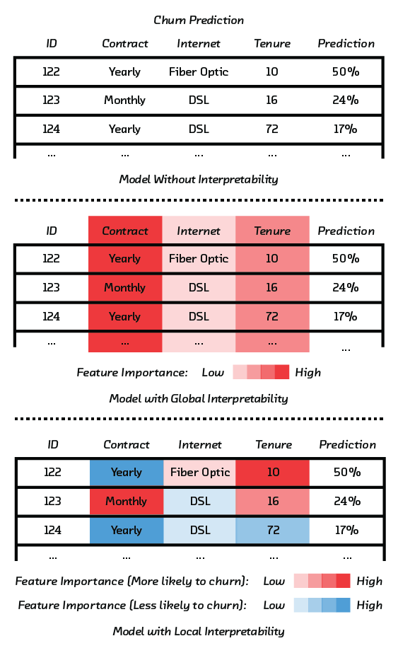
When one or more of these conditions holds, it makes our use of data safer and opens the door to new kinds of products.
Enhancing Trust
Data scientists have a well-established protocol to measure the performance of a model: validation. They train a model with perhaps 80% of their training data, then measure its performance on the remainder. By assessing the model using data it has never seen, they reduce the risk that a powerful model with a lot of flexibility will simply memorize the training data.
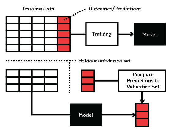
This possibility, known as overfitting, is a concern because the model will one day be deployed in the wild. In this environment, by definition, it cannot have seen the data before. An overfitted model does not capture fundamental, general trends in data and will perform poorly in the real world. Validation during training diminishes this risk. It is an absolute minimum requirement for building a trustworthy model.
But memorization or overfitting is not the only danger that lurks during training. If the training data has patterns that are not present in real-world data, an apparently good model will detect these patterns and learn to depend on them, and then perform poorly when deployed.
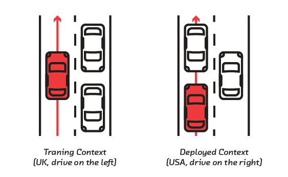
Some differences between training and real-world data can be very obvious. For example, if you train a self-driving car on public roads in a country where people drive on the left, and then deploy that car in the United States, you’re asking for trouble.
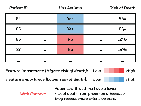
But sometimes subtler discrepancies can exist in the training data without your knowledge. A memorable example taken from a 2015 paper makes this point clearly.[1] Doctors and statisticians trained a model to predict the “probability of death” of patients suffering from pneumonia. The goal was to identify high-risk patients who should be admitted to hospital, and low-risk patients for outpatient treatment. With enough data, the conceit of machine learning is that it is able to identify patterns that doctors might miss, or that might be glossed over by crude protocols for hospital triage.
When the researchers analyzed the model (using some of the techniques we discuss in this report), they realized that the model wanted to treat patients with asthma as low-risk outpatients. Of course, the model was wrong: people with asthma are at high risk if they catch pneumonia and should be admitted to the intensive care unit. In fact, they often are, and it was this that caused a problem in the training data. Asthma patients receive excellent care when they have pneumonia, so their prognosis is better than average.
A model that captures this will perform well by the standard training metrics of accuracy, precision, and recall, but it would be deadly if deployed in the real world. This is an example of leakage: the training data includes a feature that should not be used to make predictions in this way. In this case, the model depended on a flawed assumption about the reason for the correlation between asthma and pneumonia survival.
It is obviously essential to be confident that you haven’t embedded bugs like this into a statistical model if it is to be used to make life-and-death medical decisions. But it’s also acutely important in any commercial setting. At a minimum, we need to understand how a model depends on its inputs in order to verify that this matches our high-level expectations. These perhaps come from domain experts, previous models that have worked well, or legal requirements. If we can’t do this, then we can’t be confident that it will behave correctly when applied on data that was not in the training or validation set. If we can, then we don’t just get a feeling of confidence: we gain the power to explain decisions to customers, to choose between models, and to satisfy regulators.
This trust is particularly important in machine learning precisely because it is a new technology. Rightly or wrongly, people tend to distrust novel things. Machine learning will only earn the trust of consumers, regulators, and society if we know and communicate how it works.
Satisfying Regulations
In many industries and jurisdictions, the application of machine learning (or algorithmic decision-making) is regulated. This report does not offer legal advice. To the extent that we discuss these regulations in any specific detail, we do so in Chapter 6 - Ethics and Regulations. We bring them up here for two reasons.
First, if these regulations apply, they almost always imply an absolute requirement that you build interpretable models. That is because the goal of these regulations is often to prevent the application of dangerous or discriminatory models. For example, you may be required to prove you haven’t overfitted. An overfitted model won’t work in the real world, and deploying one may hurt more than just your own bottom line. You may be required to prove that dangerous predictive features haven’t leaked in, as in the pneumonia treatment model that sent asthma patients home. And you may be required to show that your model is not discriminatory, as is the case if a model encourages a bank to lend to borrowers of a particular race more often.
In a regulated environment, it is insufficient to show that these problems were not present in your training data. You must also be able to explain the model derived from this training data, to show that they can never occur in the model either. This is only possible if the model is interpretable.
Second, even in industries where regulations don’t apply, the regulations set a standard for interpretability. They formalize and extend the question of whether the model builder trusts the model to behave as desired. In some cases they also emphasize the possibility of discrimination, which is something all data scientists should bear in mind. A model that perfectly captures the real world with 100% accuracy might seem desirable, but training data often embeds society’s biases. It may be unethical, if not illegal, to deploy a model that captures and recapitulates these biases. Interpretability allows you to reason about whether your model embeds biases before you go ahead and apply it at scale.
Explaining Decisions
Local interpretability – the ability to explain individual decisions – opens up new analyses and features, and even new products. The ability to answer the question “Why has the model made this decision?” is a superpower that raises the possibility of taking an action to change the model’s decision. Let’s consider some examples of what you can do with that capability.
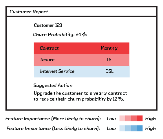
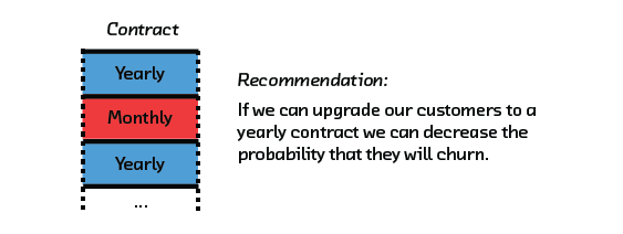
A model of customer churn tells you how likely a customer is to leave. A locally interpretable model – that is, one in which you can explain a particular prediction – offers an answer to the question of why this customer is going to leave. This allows you to understand your customer’s needs and your product’s limitations. It even raises the possibility of taking a well-chosen action to reduce the probability of churn. This problem is the focus of our prototype.
A model that predicts hardware failure in an engine or on a server is of course extremely useful. You can send an engineer out to inspect an appliance that is predicted to fail. But if the model is locally interpretable, then you can not only warn that a problem exists: you can potentially solve the problem, either remotely or by giving the engineer the reason, saving them time in the field.
A model that predicts loan repayment (or credit rating) is not only useful to the lender, it is of enormous interest to the borrower. But showing borrowers a credit rating number on its own is of limited use if they want to know what they need to do to improve it. The consumer app Credit Karma[2] allows its users to figure this out for themselves using a brute force method similar to the new algorithm that we use in this report’s prototype (see perturbation).
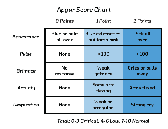
Interpretable models also tend to be more user-friendly. For example, the APGAR score used at childbirth gives an integer score out of 10. The higher the number, the healthier the newborn baby. The score is comprised of three numbers, measured by eye and combined by mental calculation. This heuristic is not machine learning, but it is algorithmic decision-making. The simplicity of the APGAR score means that, in a fast-moving environment, the obstetrician or midwife trusts its outputs and can reason about the problem with the inputs in their head: the ultimate in usability. As we discuss below in the Accuaracy and Interpretability section, this simplicity comes at a cost: the model is less accurate than a huge neural network would be. But it can often be worth trading a little accuracy for interpretability, even in contexts less extreme than hospitals.
Improving the Model
An uninterpretable model suffers from the performance and regulatory risks discussed earlier (see Enhancing Trust, and Satisfying Regulations above), and closes the door on products that take advantage of explanations (see the previous section, Explaining Decisions). It’s also much harder to improve.
Debugging or incrementally improving an uninterpretable black-box model is often a matter of trial and error. Your only option is to run through a list of ideas and conduct experiments to see if they improve things. If the model is interpretable, however, you can easily spot glaring problems or construct a kind of theory about how it works. The problems can be fixed, and the theory narrows down the possibilities for improvements. This means experiments are driven by hypotheses rather than trial and error, which makes improvements quicker.[3]
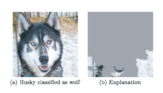
A striking example of debugging is given in the paper introducing Local Interpretable Model-agnostic Explanations (LIME),[4] the black-box interpretability technique we use in this report’s prototype. In that paper, the authors describe a convolutional neural network image classification model able to distinguish between images of wolves and Husky dogs with high accuracy. LIME’s ability to “explain” individual classifications makes it obvious that the classifier has incorrectly learned to identify not wolves and Husky dogs, but snow in the background of the image, which was more common in the training images of wolves.
Accuracy and Interpretability
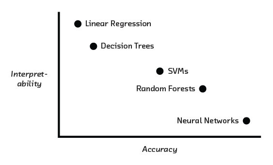
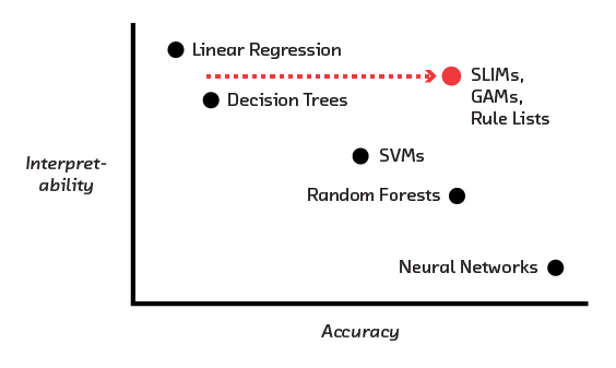
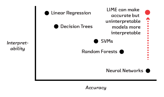
So, why not simply use interpretable models? The problem is that there is a fundamental tension between accuracy and interpretability. The more interpretable a model is, generally speaking, the less accurate it is. That’s because interpretable models are simple, and simple models lack the flexibility to capture complex ideas. Meanwhile, the most accurate machine learning models are the least interpretable.
This report is about exciting recent developments that resolve this tension. In the last few years, “white-box” models have been developed that are interpretable, but also sacrifice minimal accuracy. Separately, model-agnostic approaches that provide tools to peer inside accurate but previously uninterpretable “black-box” models have been devised. The following chapters discuss and illustrate these developments.
The Challenge of Interpretability
In the previous chapter we saw the power of interpretability to enhance trust, satisfy regulations, offer explanations to users, and improve models. But we also saw that there is a fundamental tension between these goals and a model’s ability to get decisions right. Traditionally, you can have an interpretable model or you can have an accurate model, but you can’t have both.
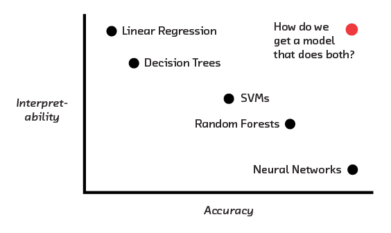
In this chapter we’ll first explain the technical reasons for this tension between interpretability and accuracy. We’ll then look at two ways to have your cake and eat it. We’ll take a tour of a handful of new “white-box” modeling techniques which are extremely interpretable by construction, but retain accuracy. We’ll then introduce the idea that is the technical focus of the report: interpretation of black-box models by perturbation and, in particular, LIME.[5]
Why Are Some Models Uninterpretable?
What is it about a model that makes it uninterpretable? Let’s first look at the gold standard of interpretability – linear models – in the context of a classification problem (the difficulties with regression models are not qualitatively different). Suppose we’re classifying borrowers as likely to repay or not. For each applicant we will have access to two pieces of information: their annual income, and the amount they want to borrow. For a training sample we also have the outcome. If we were to plot the training data, we might see something like this:
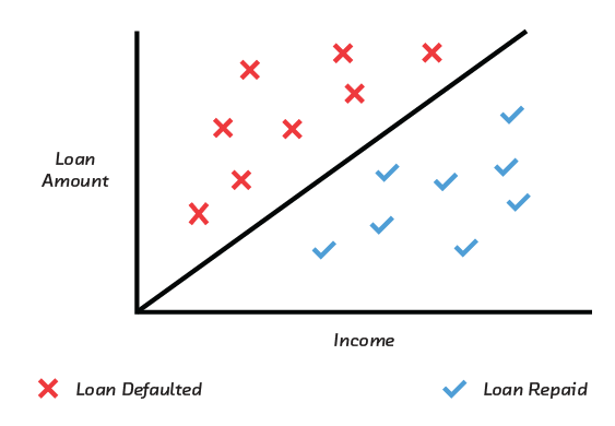
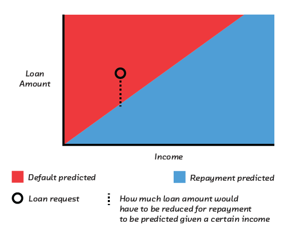
At a high level, this training data shows that people who repay tend to earn a lot and borrow a little. But the details are important. You can draw a straight line on this chart that separates the repayers and non-repayers. You can then build an accurate model by simply asking the question, “Is the applicant above or below the line?” Formally, this is a linear model; i.e., one in which the predicted repayment probability is a linear function of income and loan amount.[6] In other words:
Probability of repayment = A × income + B × loan amount
where the coefficients A and B are two numbers.
Such a model is interpretable. A is just a number, and not a function of any
other number, so we can easily check whether it is positive. If it is, we can
know with certainty that repayment probability increases with income in our
model. This directional behavior probably matches the expectations of domain
experts, which is reassuring to us and to regulators. The structure of the
equation means that this trend will always be true. It’s mathematically
impossible for some obscure combination of income and loan amount to imply that
repayment probability decreases with income. That mathematical certainty means
we can be confident that there is no hidden behavior lurking in the model. Our
trust in the model is high. And we can use the numbers A and B to tell a
borrower why we think they are unlikely to repay in precise but plain words
(e.g., “Given your income, you are asking to borrow $1,000 too much.”).
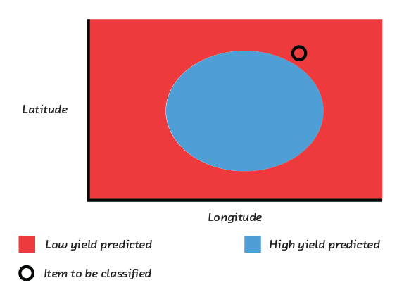
Let’s look at a tougher problem. Suppose we plot the longitude and latitude of temperature sensors in a field, and mark with a check or cross whether the yield of corn was high or low:
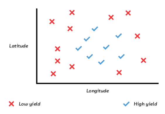
As you can see, there is no way to draw a straight line that separates the high-yield and low-yield areas of this field. That means it will be impossible to build an accurate and maximally interpretable linear model solely in terms of latitude and longitude.
The obvious thing to do in this particular case would be to “engineer” a feature that measured distance from the center of the field (which is a function of both longitude and latitude). It would then be simple to build a model in terms of that single derived feature. Feature engineering, however, is time-consuming and can require domain expertise. Let’s suppose we didn’t have the time or expertise. In that case we might graduate from a linear model to a Support Vector Machine (SVM).
An SVM essentially automates the process of engineering our “distance from the center of the field” metric. It does this by distorting the 2D surface on which the points in the previous figure sit into three or more dimensions, until it is possible to separate the high- and low-yield areas of the field with a plane.
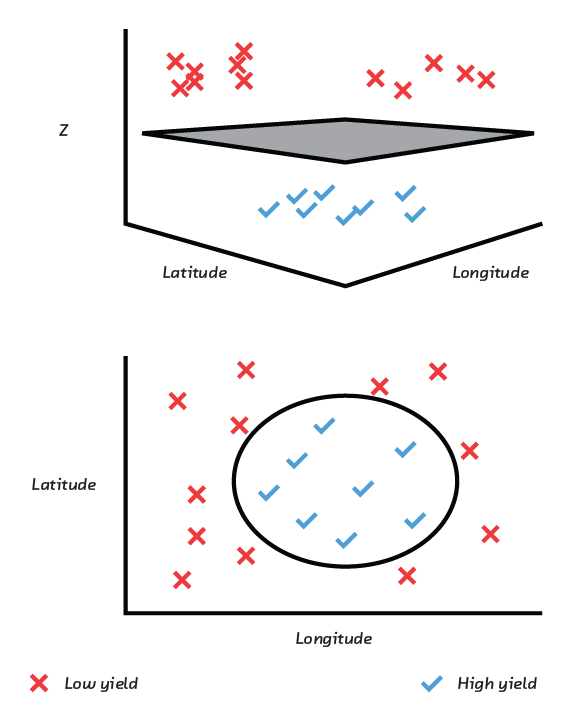
This model will be accurate, but the distortion of the inputs means that it no longer operates in terms of our raw input features. We cannot write down a simple equation like our loan repayment equation that allows us to say with confidence exactly how the model responds to changes in its inputs in all parts of the field. There is an equation, but it’s longer and more complicated. It has therefore become harder to give a simple explanation of why an area is predicted to have high or low yield. If a farmer wants to know whether moving to the west will increase yield, we have to answer that it depends on how far north you are. Our model’s internal structure is a step removed from the relatively intuitive raw input.
If we take one more step up in problem and model complexity, the internal structure of the model gets still more removed from the input. A neural network used to classify images does an exponentially large number of transformations similar to but more complex than the single one performed by an SVM. The equation it encodes will not only be very long, but almost impossible to reason about with confidence.
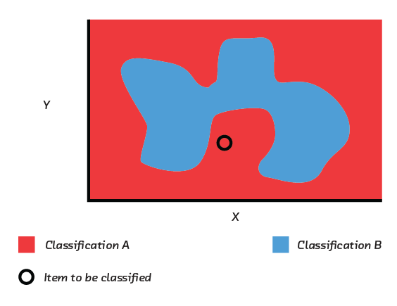
A random forest model is often used where the problem is hard and the main concern is accuracy. It is an ensemble, which means that it is in a sense a combination of many models. Although the constituent models are simple, they combine in a way that makes it extremely difficult to summarize the global model concisely or to offer an explanation for a decision that is locally true. It is all but impossible to rule out the possibility that the model will exhibit nonsensical or dangerous behavior in situations not present in the training data.
White-box Models
The least interpretable models, such as neural networks, are free to choose from an almost infinite menu of transformations of the input features. This allows them to divide up the classification space even if it is not linearly separable. New white-box models have a smaller menu of transformations to choose from. The menu offers a big boost in freedom to classify with accuracy, but is carefully chosen with interpretability in mind too. Generally speaking, this means that the model can be visualized or is sparse. Visualization is one of the most powerful ways of immediately grasping how a model works. If it is not possible, then the model is much harder to interpret. Models that are sparse, meanwhile, are mathematically simple in a way that raises the possibility that they can be written down as a set of simple rules.
GAMs
Generalized additive models (GAMs) are a great example of this carefully controlled increase in model flexibility. As we saw earlier, a linear classification model assumes that the probability a given piece of data belongs to one class rather than another is of the form:
Ax + By + Cz
where the coefficients A, B, and C are just constant numbers, and x, y, and z are
the input features. A GAM allows models of the form:
f(x) + g(y) + h(z)
where f and g are functions. This model is “generalized” because the
constant coefficients have been replaced with functions – in a sense, the
constant coefficients are allowed to vary, which gives the model more
flexibility. But it is “additive” because the way in which f(x), g(y), and
h(z) are combined is constrained, which means the flexibility is not total.
In particular, the functions f, g, and h are each functions of one of the
features only, and the terms f(x), g(y), and h(z) must be combined by
simple addition.
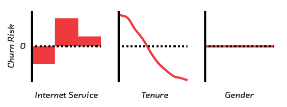
This careful loosening of the constraints of linear models allows higher
accuracy, but retains the ability to construct partial dependence plots.
These are simply graphs of f(x), g(y), and h(z) that allow us to
visualize the behavior of the model. These graphs can be examined to ensure
that there are no dangerous biases lurking in the model or, if necessary, to
demonstrate to a regulator that a model responds monotonically to a
particular feature.[7]
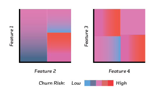
GA^2^2Ms extend GAMs by allowing pairwise interacti^ons, or models of the form:
f(x) + g(y) + h(z) + p(xy) + q(yz)
That is, they allow a tightly constrained version of the kind of feature
engineering we saw in the field yield example earlier. There is in principle
nothing to stop us introducing a model with another term, r(xyz), but GA^2^Ms
stop here for a very good reason: you can make a partial dependence plot of
p(xy) by drawing a heatmap, but it is extremely difficult to make a partial
dependence plot of three variables. It is the partial dependence plots that
give the model its interpretability.
We’ve described a situation with just three features, x, y, and z. But
it’s more common to have many more features. This raises the possibility of
exponentially many pairwise terms. For example, with 50 features there are over
a thousand possible pairwise terms. Trying to inspect all these plots would
diminish interpretability rather than enhancing it. For this reason, GA^2^Ms
include only the k pairwise terms that most improve accuracy, where k is a
small number determined like any other hyperparameter.[8]
Rule Lists
Rule lists are predictive models that learn simple flow charts from training
data. The models are made up of simple if...then...else rules that partition
the input data. These rules are the building blocks of rule lists. For
example, it’s possible to predict survival of passengers on the Titanic using
a rule list like this:
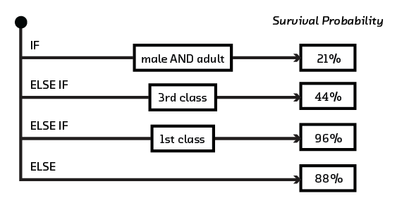
Rule lists are special cases of decision trees, where all the leaves are on the same side of the tree. As such, they are highly interpretable.
Bayesian rule lists (BRLs)[9] and falling rule lists (FRLs)[10] are recent instantiations of this general approach. Given a catalog of rules learned from data, BRLs use a generative model to select a smaller subset of highly probable rules that best describe the data the rules were learned from. In the case of FRLs, the model is structured so that the selected rules are ordered by importance, which allows users to more easily identify the important characteristics.
Rule list methods are a good fit for categorical data. Numerical data can be discretized, but if the statistical relationships among input attributes are affected by discretization, then the decision rules learned are likely to be distorted.
SLIMs
The APGAR score for newborn infants (see Explaining Decisions) is calculated by assigning scores of 0, 1, or 2 to five attributes of the baby and adding them up:
APGAR = appearance + pulse + grimace + activity + respiration
As we discussed, the fact that this score can be calculated quickly and reasoned about easily is an important feature. Scores like this are in widespread use in clinical medicine. But this extreme simplicity necessarily comes at the expense of accuracy.
In the same way GA^2^Ms use a tightly controlled freeing up of a linear classifier to increase accuracy, Supersparse Linear Integer Models (SLIMs)[11] make a small change to scoring systems to increase their accuracy. That change is to permit each attribute to be multiplied by an integer coefficient. With this additional freedom, the APGAR score might become:
APGAR = 5 appearance + 3 pulse + 2 grimace + 7 activity + 8 respiration
A score like this is almost as easy to work with as the original APGAR score, and potentially hugely more accurate. The challenge is figuring out how to choose the numbers. SLIMs cast this problem as a supervised machine learning problem and use the tools of integer programming to ensure the coefficients are round numbers.
Black-box Interpretability
If you won’t or can’t change your model, or you didn’t make it and don’t have access to its internals, white-box approaches are not useful. In this extremely common situation, you need an approach that allows you to interpret a black-box model. Thanks to recent research, this is not only possible, but relatively simple.
Until recently, the usual way to interpret a black-box model was to train two models: the uninterpretable, highly accurate model that you use in production, and a shadow interpretable model you use solely to learn about the system. The shadow model is trained not on real training data, but on simulated data generated by the uninterpretable, accurate model. It’s therefore a caricature of the truth and, at a high level, may capture some of the broad strokes of the model. By inspecting the interpretable shadow model, you can offer explanations.
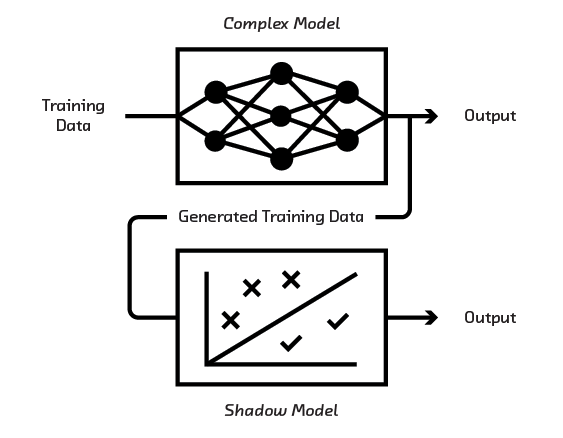
The problem is that the shadow model is not only simplistic by construction. Its explanations can be misleading in ways you have no easy way of knowing. Inferences drawn from it are dubious, and come with no statistical guarantees about how wrong they could be. Simply put, you can offer explanations for the production model’s decisions, but you have no way of knowing if those explanations are correct.[12] Additionally, you now need to build and maintain two models, which can be a significant engineering burden.
Perturbation
Perturbation is a model-agnostic interpretability technique that requires you to build and maintain only one model. This is your production model. It can be as complicated and uninterpretable as is justified by your dataset and performance requirements. Despite this, the strategy offers a more faithful description of the uninterpretable model than the interpretable shadow model technique described in the previous section.
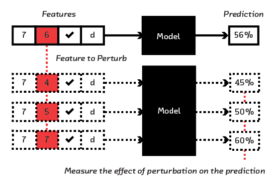
The basic idea is simple, and is probably exactly what you’d do if you were asked to figure out how a black-box system worked. The input is perturbed, and the effect of that perturbation on the output is noted. This is repeated many times, until a local understanding of the model is built up.
Let’s look at a real-world example of the application of this basic idea in its simplest, most manual form. The website Credit Karma offers a Credit Score Simulator. At first the simulator shows the user their current score. The user can then change one of the two dozen or so inputs, to see what the effect is. The natural thing to do is to try changing them all, one at a time, to see which has the biggest effect.
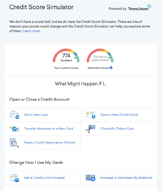
Credit score is a nonlinear model; two people can open the same new credit card and it can have very different effects on their credit score. This means it is impossible to summarize the model globally by saying something like “Lose 10 points per open credit card.” But if a particular user of the Credit Score Simulator discovers their score goes down by 10 points when they propose opening a new credit card, that is a valid explanation of the behavior of the model locally, in the vicinity of that user in feature space.
LIME
Local Interpretable Model-agnostic Explanation (LIME)[13] formalizes the perturbation technique described in the previous section. It’s exciting because it provides a simple method to interpret arbitrary black-box models. The algorithm is computationally simple, and the public reference implementation is a drop-in addition to many machine learning pipelines.
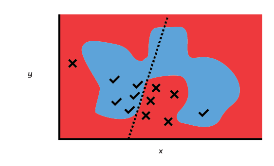
LIME takes as input a trained model and the particular example whose classification you want to explain. It then randomly perturbs the features of the example, and runs these perturbed examples through the classifier. This allows it to probe the surrounding feature space and build up a picture of the classification surface nearby.
It probes the classifier’s behavior in this way a few thousand times, and then uses the results as training data to fit a linear model. The training examples are weighted by distance to the original example. The linear model can then be interpreted as usual to extract explanations like “You will decrease your credit score by 10 points if you open a credit card.” These explanations are locally faithful; i.e., they are applicable in the region near the original example.
In a way, this approach is similar to the shadow model approach: the “true” model is used to generate training data for a simpler, interpretable model. But while the shadow model offers a supposedly global explanation that is wrong in unknown ways, LIME offers a local explanation that is correct.
LIME is an exciting breakthrough. It’s an extremely simple idea (the preceding explanation glosses over mathematical detail, but is conceptually complete). It allows you to train a model in any way you like and still have an answer to the local question, “Why has this particular decision been made?” We used LIME to build the prototype for this report.
Extensions and Limitations
LIME is well suited to tabular data. It perturbs categorical features by sampling from their distribution in the training data, and it perturbs continuous features by sampling from a normal distribution.
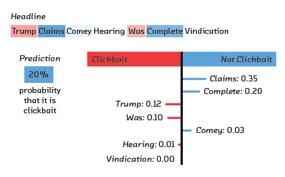
How to meaningfully perturb unstructured input such as images or text is less obvious. For text, the reference implementation offers two perturbation strategies. It can either delete words, or replace them with an unknown token. Using these strategies, the “local” region around the example is the set of trial documents made by omitting words from the original. By running these trial documents through the black-box classifier, LIME can learn which words in the original document are “responsible” for the original classification, and assign them quantitative importances.
These importances can be used to label the words in a document that are “responsible” for its classification (by topic, sentiment, etc.). Assuming the model is accurate, it is presumably relying on some of the same things a human reader is looking for. If you’re the author of the text, you might therefore find it useful to know which parts of your writing are attracting the model’s attention. If you’re the creator of the model, you might find it reassuring (or alarming) to learn the words your model depends upon.
We applied LIME to a black-box text classifier and saw sensible results. The model, a recurrent neural network to classify text as clickbait or not, was truly a black box to us.[14] We found it online and deliberately avoided reading about its structure. Nevertheless, we were able to use LIME to probe it, and build up some trust that it was paying attention to reasonable words.
The image perturbation strategy suggested by the creators of LIME is qualitatively similar. The image is divided up into high-level “superpixels,” which are zeroed out at random during perturbation. The result is the same: an explanation that says which part of the image is responsible for the behavior of the black-box model.[15]

While LIME is designed with local explanation in mind, with enough explanations in hand, you can begin to build up in your head a global picture of the model. But doing this is like playing Battleship: you try examples at random, and dwell in interesting places when you find them. The creators of LIME also introduced SP-LIME, an algorithm to select a small number of well-chosen real examples from a dataset. The algorithm greedily selects examples whose explanations are as different as possible from each other. The result is a small number of examples that, along with their explanations, give the big picture.[16]
Finally, it’s important to note that the LIME approach has fundamental limitations. Whether it is used to explain a classifier of tabular, text, or image data, LIME gives explanations in terms of the raw input features. If those features are not interpretable, then LIME will not help. For example, if the initial input to a model is an uninterpretable text embedding, LIME will not offer an explanation that makes sense to humans.
Also, as with any attempt to attribute causal relationships to data, there are dangers of confusing correlation and causation. This risk, which exists throughout machine learning, is equally if not more acute when using LIME. It is easy to read LIME’s explanations as saying things like “This cable customer is going to churn because they do not have TV service,” which may be a misinterpretation. The risk of this is highest when when the supposed causal relationship seems to confirm your expectations.
Global black-box interpretation with FairML
FairML is an open source tool released by Julius Adebayo when he was a member
of the Fast Forward Labs team. It is similar to LIME in the sense that it
probes a black-box model by perturbing input, but it provides a single global
interpretation that assigns an importance to each feature. As with a shadow
model, this may gloss over important details, but for the purposes of auditing
a model for harmful global biases it is a great tool. For example, it can be
used to measure the extent to which a model depends on “protected features”
that, from a legal and ethical point of view, should make no difference to its
output (see <
SHAP
Following the release of LIME, there has been continuous research focused on improving accuracy as well as the user experience tooling for explaining blackbox models. One such contribution, which has rapidly become an widely used, is SHAP [18]. SHAP stands for SHapley Additive exPlanations and its primary contribution is the introduction of a game theoretic foundation (Shapley values) for assigning feature importance values for each prediction produced by a model. Shapley values (introduced by Lloyd Shapley in 1953) are a method for fairly assigning credit to participants in a cooperative multiplayer game based on their contributions to the overall game outcome.
To compute the Shapley value for a given player, we compute each outcome where the player was present and compare it to the outcome where they were not present. For a game consisting of N players, there is a large surface of outcome combinations (N!) where each player is present or absent, making the computation of Shapley values computationally expensive.
More importantly, the Shapley value approach for assigning credit is fair because it adheres to a list of certain mathematical properties (Efficiency, Symmetry, Linearity, Anonymity, Marginalism) beyond the scope of this writeup. When applied to model explanations (assigning credit for each feature in a prediction), the integration of the Shapley approach yields two valuable properties
- local accuracy (an approximate model used to explain the original model should match the output of the original model for a given input)
- consistency (if the original model changes such that a feature has a larger impact in every possible ordering, then its attribution should not decrease)
In their paper, [19] the authors of SHAP show that most approaches to explaining black box models (LIME, DeepLIFT, Relevance Propagation) can be categorized as additive feature attribution methods and that a Shapley value approach is the only approach that guarantees the local accuracy and consistency properties within the category. The authors also show through experiments how these properties help to avoid unintuitive results that can sometimes be observed with non-shapely methods like LIME.
SHAP is implemented as a python library with an easy to use interface and a set of useful visualizations. To address the complexity of computing Shapley values, the authors implement optimizations that take advantage of the structure of specific models. For example, the SHAP TreeExplainer is optimized for tree based models (XGBoost/LightGBM/CatBoost/scikit-learn/pyspark models) while DeepExplainer and GradientExplainer are optimized for neural networks. However, SHAP remains slow when used in model agnostic mode (KernelSHAP).
The code below shows how to generate a list of Shapley values that quantify the effect of each feature on the model prediction.
import shap
# model is a sklearn decision tree model applied to the churn dataset used in the prototype
explainer = shap.TreeExplainer(model)
shap_values = explainer.shap_values(X_test)
The SHAP python library also provides helpul visualizations that further illustrate the global and local impact of each feature.
# Local explanation for single instance
shap.force_plot(explainer.expected_value, shap_values[0,:], X_test.iloc[0,:], matplotlib=True)

# Global explanation for all instances in test set
shap.summary_plot(shap_values, X_test)
shap.summary_plot(shap_values, X_test, plot_type="bar")

force_plot visualization which shows the local feature importance for each a given data instance.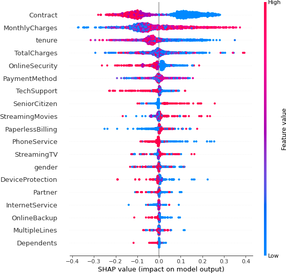
summary_plot visualization which shows the global feature importance entire test set.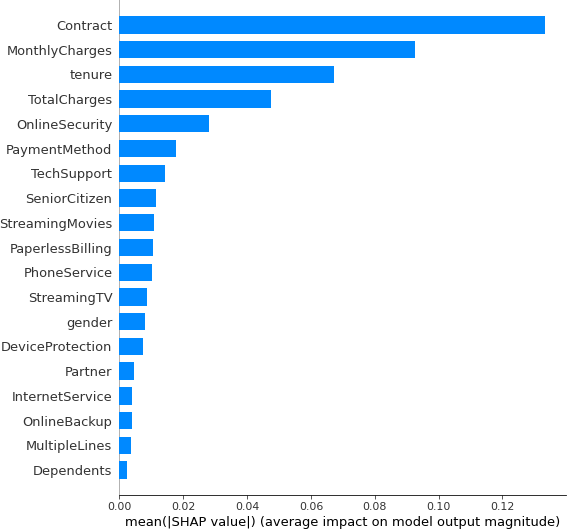
Prototype
In order to bring interpretability to life, we chose to focus our prototype on LIME’s ability to explain individual algorithmic decisions.
Alongside the rate at which a business acquires customers, the rate at which it loses them is perhaps the most important measure of its performance. Churn is well defined for an individual customer in a subscription business. This makes it possible to collect training data that can be used to train a model to predict whether an individual customer will churn. Our prototype uses LIME to explain such a model.
If the relationship between the attributes of a customer and their churning is causal, and the model that predicts churn from these attributes is accurate, LIME raises an interesting possibility. If you can explain the model’s prediction for a customer, you can learn why the customer is going to churn, and perhaps even intervene to prevent it from happening.
Establishing a causal relationship can be tricky, and not all attributes can be changed. In such cases it may not make sense or be possible to intervene. For example, if a model predicts a customer is going to churn because they are over a certain age, there’s not much you can do about it. But even if it’s not possible to intervene, the ability to group customers according to the attributes that are most concerning is a powerful way to introspect a business. It may bring to light groups of customers you want to focus on, or weaknesses in the product.
Using the churn model in this way depends on it being interpretable, but a complicated business with thousands of customers, each of whom it knows a lot about, may need a model using techniques such as uninterpretable random forests or neural networks.
This is a job for model-agnostic interpretability. By applying LIME to an arbitrarily complicated model, we can have it both ways: an accurate model describing an intrinsically complicated dataset, that is also interpretable.
Customer Churn
We used a public dataset of 7,043 cable customers, around 25% of whom churned.[20] There are 20 features for each customer, which are a mixture of intrinsic attributes of the person or home (gender, family size, etc.) and quantities that describe their service or activity (payment method, monthly charge, etc.).
We used scikit-learn to build an ensemble voting classifier that incorporated
a linear model, a random forest, and a simple neural network. The model has an
accuracy of around 80% and is completely uninterpretable.
Applying LIME
As described above in Chapter 3, LIME explains the classification of a particular example by perturbing its features and running these perturbed variations through the classifier. This allows LIME to probe the behavior of the classifier in the vicinity of the example, and thus to build up a picture of exactly how important each feature is to this example’s classification.
Before it can do this, LIME needs to see a representative sample of training data to build an “explainer” object. It uses the properties of this sample to figure out the details of the perturbation strategy it will eventually use to explain an individual classification. This process is a little fiddly in the reference implementation that we used,[21] because it requires some bookkeeping information about categorical features. But once the explainer has been instantiated it can be saved for future use, alongside the model.
The explainer then requires two things to explain an individual classification: the features of the example to be explained, and the classifier (in the form of a function that takes the features as input and returns a probability).
This yields an “explanation” for a given example and class, which is just a list of weights or importances for all or a subset of the features. These are a measure of the sensitivity of the classifier to each feature, in the local region of the particular example. A large positive number means that the particular feature contributes a lot toward the example’s current classification. A large negative number, on the other hand, means that a feature’s value implies that the example belongs in a different class. Numbers close to zero indicate that a feature is unimportant.
This code will give us a list of (feature, importance) tuples:
from lime.lime_tabular import LimeTabularExplainer
explainer = LimeTabularExplainer(training_data=X,
                             training_labels=y,
                             feature_names=feature_names,
                             class_names=class_names)
# clf is the churn classifier we want to explain
e = explainer.explain_instance(customer, clf.predict_proba)
print(e.as_list())
For our use case, we are interested in the features with the largest positive importances, which tell us which features are most responsible for the model thinking the customer will churn.
Computational resources
In order to comprehensively probe the area around an example, LIME needs to perturb every feature, and then build a linear model with the same features. This means the time it takes to construct an explanation is most sensitive to the number of features in the data.[22] In our tests LIME explained a classification of our model, which had 20 features, in around 0.1s on a commodity PC. This allowed for a responsive user interface. We also applied our prototype to a proprietary churn dataset with 100 features. That increased the time required for an explanation to 1s on the same hardware. We could have increased the power of the hardware or reduced the number of perturbations below the standard 5,000 to speed this up if necessary.
We wrapped our dataset, scikit-learn classifier, and LIME explainer in a
standard Python Flask web API. This allows frontend applications to get
customer data, the corresponding churn probabilities, and the LIME explanations
for those probabilities.
Product: Refractor
The Product Possibilities of Interpretability
As the use of machine learning algorithms increases, the need to understand them grows as well. This is true at both a societal and a product level. As algorithms enter into our workplaces and workflows, they appear mysterious and a bit intimidating. Their predictions may be precise, but the utility of those predictions is limited if we cannot understand how they were reached. Without interpretability, algorithms are not great team players. They are technically correct but uncommunicative.
Interpretability opens up opportunities for collaboration with algorithms. During their development, it promises better processes for feature engineering and model debugging. After completion, it can enhance users’ understanding of the system being modeled and advise on actions to take.
For our prototype, we wanted to explore how that collaboration through interpretability might look. We chose an area, churn probability for customers of an Internet service provider, where the collaboration payoff is high. Making the churn prediction is the kind of problem machine learning excels at, but without an understanding of what features are driving the predictions, user trust and ability to take action based on the model are limited. With interpretability, we can break out of those limitations.
Our prototype, Refractor, guides you through two levels of interpretability, from a global table view of customers to an exploration of the effects of different features on an individual user. The process of building the prototype was also a movement between, and eventually a balancing of, those two levels.
Global View: Understanding the Model
LIME is focused on local explanation of feature importance through feature perturbation. It may initially seem a strange choice, then, to use it in a globally oriented view. The stacked local interpretations, however, coalesce into a powerful global representation of how the algorithm works. For many complex algorithms, this is the only kind of global view you can have.
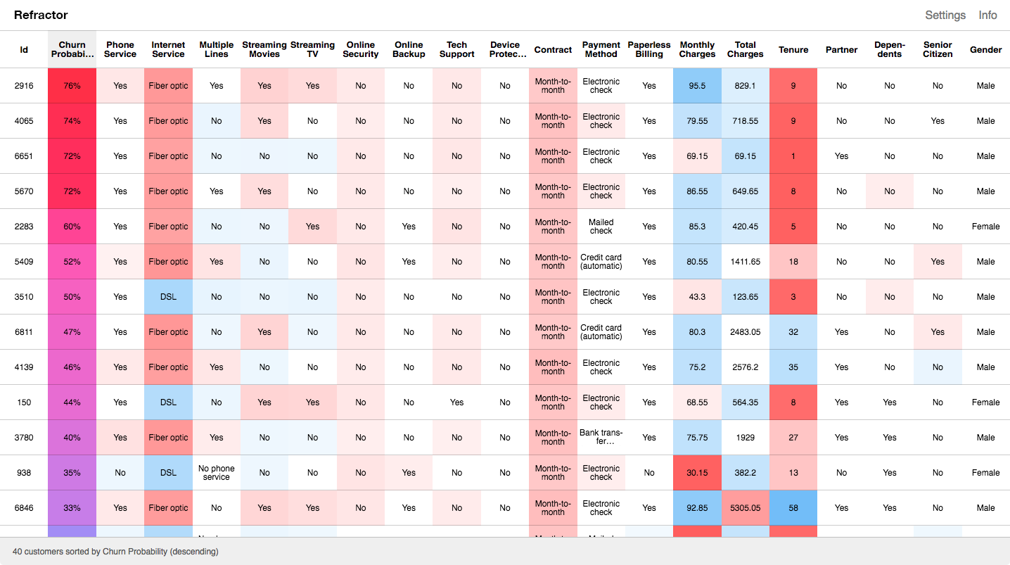
Machine learning models are powerful because of their ability to capture nonlinear relationships. Nonlinear relationships cannot be reduced to global feature importance without significant information loss. By highlighting local feature importance within a table view, you do see important columns begin to emerge, but you can also observe patterns, like discontinuities in a feature’s importance, that would have to be averaged out if feature importance was globally calculated.
The table, as a sort of global view of local interpretability, highlights how interpretability depends on collaboration. The intuitive feel a user builds up from scrolling through the highlighted features depends on our ability to recognize patterns and develop models in our heads that explain those patterns, a process that mirrors some of the work the computer model is doing. In a loose sense, you can imagine that the highlighted features give you a glimpse of how the model sees the data – model vision goggles. This view can help us better debug, trust, and work with our models. It is important to keep perspective, however, and remember that the highlighted features are an abstracted representation of how the model works, not how it actually works. After all, if we could think at the scale and in the way the model does, we wouldn’t need the model in the first place.
Local View: Understanding the Customer
While the table view is a powerful interface, it can feel overwhelming. For this prototype, we wanted to complement it with an individual customer view that would focus on actions you could take in relation to a specific customer.
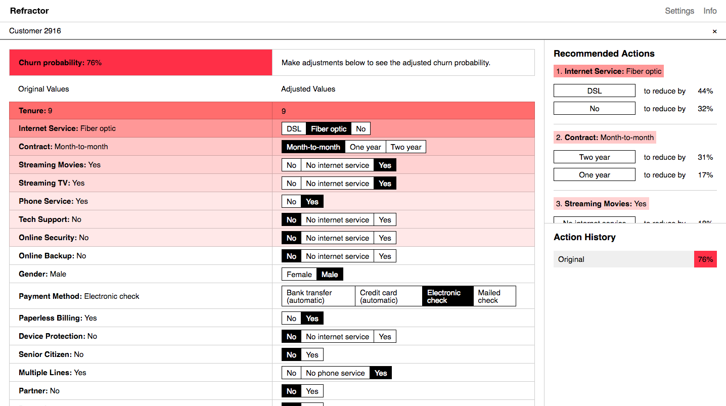
Free of the table, we are now able to change the displayed feature order. The obvious move is to sort the features by their relative importance to the prediction. In the vertical orientation, this creates a list of the factors most strongly contributing to the customer’s likelihood of churning. For a customer service representative looking for ways to decrease the chance the customer will leave, this list can function as a checklist of things to try to change.
Because this sorting is an obvious move, it’s easy to undervalue its usefulness. It is worth remembering that without LIME (or a different interpretability strategy), the list would remain unsorted. You could manually alter features to see how the probability changed (as described earlier in the Credit Karma example), but it would be a long and tedious process.
The implicit recommendations of the feature checklist are built upon with further information. The recommendation side panel highlights the top three “changeable” features (e.g., not a customer’s age) and uses the model to calculate the percent reduction in churn probability that changing each feature would have.
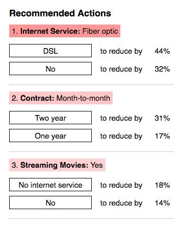
As the user follows these recommendations, or explores by changing other feature values for the individual customer, we not only calculate the new churn prediction, we also calculate the weights based on the new feature set. This ability to change one feature value and see the ripple effect on the importance of other features once again helps the user build up an intuitive feeling of how the model works. In the case of a customer service representative with an accurate model, that intuitive understanding translates to an ability to act off of its insights.
Product Tension: Focus vs. Context
As we developed the global and local interfaces of the prototype, we constantly engaged with a tension between providing the user with context and providing a focused and directed experience. This tension will arise any time you are adding interpretability to a model, and requires careful consideration and thought about the purpose of your product.
In the early stages of prototype development we kept all of the features visible, using color and ordering to emphasize those with higher importances. As we probed how a consumer product using LIME might work, we explored only showing the highest-importance features for each customer. After all, if you’re a customer service representative concerned with convincing a user to stay, why would you need to know about features that, according to the model, have no discernible effect on the churn prediction?
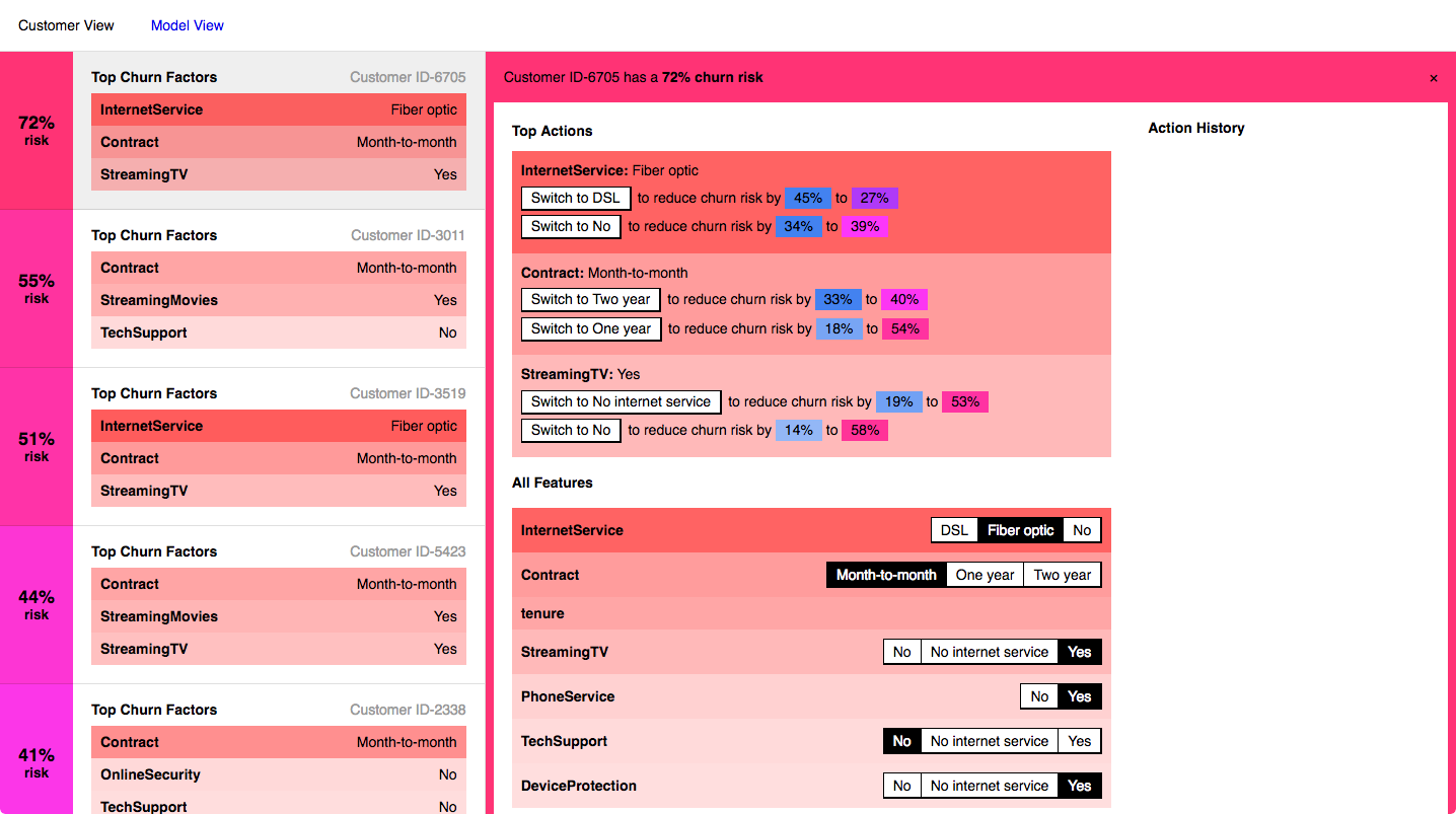
We experimented with interfaces emphasizing just the top features, and they did have the benefit of being more clear and focused. However, the loss of context ended up decreasing the user’s trust and understanding of the model. The model went back to feeling more black box-like. Being able to see which factors don’t make contributions to the prediction (for example, gender) and checking those against your own intuitions is key to trusting the features that are rated of high importance.
Having seen the importance of context, we decided to focus our prototype on that, while also dedicating some space to a more focused experience. In the individual view, this means that along with the full list of features we show the more targeted recommendation panel. For a customer service representative, this recommendation panel could be the primary view, but providing it alongside the full feature list helps the user feel like they’re on stable ground. The context provides the background for users to take more focused action.
Collaborating with Algorithms
Trust is a key component of any collaboration. As algorithms become increasingly prevalent in our lives the need for trust and collaboration will grow. Interpretability strategies like LIME open up new possibilities for that collaboration, and for better and more responsible use of algorithms. As those techniques develop they will need to be supported by interfaces that balance the need for context with a focus on possible actions.
Landscape
In this chapter we discuss specific real-world applications of interpretability, based on interviews with working data scientists. We also assess the offerings of vendors who aim to help data scientists and others build interpretable models.
Interviews
In our interviews and discussions with data organizations where interpretability is a concern, we found that most chose white-box models in order to maintain interpretability. These companies are so concerned with knowing how a model produced a given result that they are willing to potentially trade off the accuracy of the result.
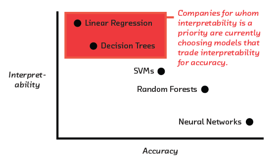
Some companies using black-box models were unwilling to provide details about interpretability, or the applications of their models. We suspect that their unwillingness to discuss may be rooted in regulatory concerns. Specifically, at least until there are regulatory rulings to bring certainty, it remains unclear whether a black box-compatible tool such as LIME is sufficient to meet regulations requiring explanation of model behavior.
Recommendation Engines
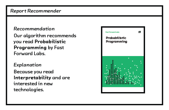
Recommendations are a straightforward, relatively low-risk, user-facing application of model interpretation. In the case of product recommendations, users may be curious why a certain item was recommended. Have they purchased similar products in the past? Did people with similar interests purchase that product? Do the recommended products share certain features in common? Are the products complementary? Or is there some other reason? This explanation builds trust with the users (especially if the recommendations are good!) by showing them what’s happening behind the scenes.
Credit Scores
Customer credit evaluation uses interpretable models extensively. When evaluating a customer’s credit score, and particularly when denying a customer credit, it is necessary to explain the basis for the credit decision. Traditionally this is done with simple models that are inherently interpretable. Technologies like LIME permit the use of more complex and potentially more accurate models while preserving the ability to explain the reasons for denial or assigning a particular score. The ethical considerations associated with these kinds of decisions are discussed in Chapter 6 - Ethics and Regulations.
Customer Churn Use Case
As we demonstrate with our prototype, churn modeling is another clear case for interpretability. Knowing when a user is likely to defect is helpful on a number of levels. It’s useful for predicting revenue streams, testing effectiveness of promotions or marketing campaigns, and evaluating customer service efficacy. Interpretation of churn models compounds their utility. For example, as shown in our prototype, interpretation of churn data can explain why a given customer or set of customers are likely to churn. This information offers customer service personnel the ability to retain more customers by helping them identify those who may be considering taking their business elsewhere and offering insights into the reasons driving that prediction. Armed with this knowledge, the representative can offer a customer a promotion or better-suited product and improve the chance of their staying.
Fraud Detection
Predictive models can help identify fraudulent activities such as credit or bank transactions, or insurance claims. Flagging these transactions creates a high-risk list for risk management personnel (or criminal activity investigators, including police) to investigate further. Models that provide deeper understanding than a simple fraud flag or likelihood indicator and show investigators the reasons a transaction was flagged can lead to improvements in resource allocation and greater effectiveness in catching fraudsters. This additional context can help investigators to dismiss some flagged transactions as appropriate, quickly eliminating false positives and enabling them to focus investigative resources elsewhere. It may also help them to plan investigations, providing hints on where to look for evidence.
Anomaly Detection
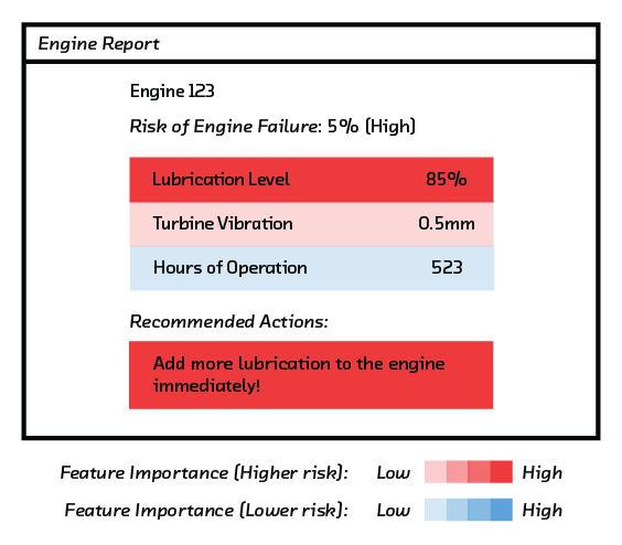
Predictive models can be used to predict failures in a variety of systems, including computer systems and networks, or even mechanical systems or industrial plants. Airlines have used such models to schedule maintenance on airplane engines that are predicted to have trouble. This is helpful, but interpretable models can identify the reason a system is likely to experience a failure and suggest targeted interventions to remedy, mitigate, or entirely prevent the problem. Fed back into the system, this understanding can suggest improvements to the design of more robust new systems.
Healthcare
Models that support diagnosis or treatment must be interpretable in order to be safe. The danger of subtle problems with training data is particularly acute because ethical constraints make it difficult to modify or randomize care in order to collect unbiased data. The requirement to “do no harm” can only be fulfilled with certainty if the model is understood. And as in the case of churn analysis, good models whose decisions can be explained offer hints toward (or even outright instructions for) the best next steps for a given case.
Data Science Platforms
White-box models are interpretable by design. At the time of writing of this report, there were no vendors focused on providing interpretability solutions for black-box models. Interpretability-as-a-service is not available (yet), but it is a capability within some data science platforms.
Data science platforms seek to provide one central place for data science work within an organization. They promise to increase collaboration and cross-pollination within and across teams, as well as building transparency into data science work. They aim to offer infrastructure and software solutions to common bottlenecks in the data science workflow that quickly deliver reliable, reproducible, and replicable results to the business. Some data science platforms aspire to enable non-data scientists (e.g., software engineers, business analysts, executives) to do data science work.
Platforms should therefore be evaluated on their solutions to common bottlenecks in the entire data science workflow. In addition to interpretability, these include:
- Easy access to scalable computing resources (e.g., CPUs, GPUs)
- Management and customization of the compute environment, software distributions, libraries
- Access to open source tools and libraries (e.g., Python, R,
scikit-learn) - Data exploration and experimentation
- Code, model, and data versioning
- Path from prototype to model deployment
- Monitoring tools for deployed solutions
- Collaboration, communication, and discovery tools
Domino Data Lab’s service, for example, does not include off-the-shelf interpretability solutions, but it is nevertheless a high-quality data science platform.[23]
Still, as we emphasize throughout this report, interpretability is an important consideration. As trained data scientists become less involved in model selection, training, and deployment, we need tools to enable us to trust models trained automatically or by non-experts. The following offerings stand out for their interpretability solutions.
H2O.ai
H2O.ai (Mountain View, CA; founded 2011; Series B Nov 2015) provides an open source platform for data science, including deep learning, with an enterprise product offering. The developers summarized their knowledge and offering with regard to interpretability in “Ideas on Interpreting Machine Learning,” a white paper published by O’Reilly.[24] Their work includes a twist on LIME called k-LIME. k-LIME trains k linear models on the data, with k chosen to maximize R^2^ across all linear models. This approach uncovers regions in the data that can be modeled using simpler linear, interpretable models, offering a solution that sits comfortably between global and local interpretability.
Of all the platforms evaluated for this report, H2O’s developers have thought the most extensively about interpretability and how to best explain complex, nonlinear relationships between inputs (i.e., features) and outputs (i.e., labels). In addition, they are actively working on novel solutions to aid data exploration and feature engineering, including visualization tools to help humans, who are adapted to perceive a three-dimensional world, understand relationships in higher-dimensional spaces.
DataScience.com
DataScience.com (Culver City, CA; founded 2014; Series A Dec 2015) released its data science platform in October 2016 and Skater (a Python library for model interpretation),[25] in May 2017. Skater includes implementations of partial dependence plots and LIME. The team at DataScience.com developed their own in-house sampler for LIME with the aim of improving the efficiency of the algorithm. The company provides robust solutions for both global and local interpretability as part of its data science platform and services offering. We welcome its decision to open-source Skater, a meaningful contribution to the data science community.
DataRobot
DataRobot (Boston, MA; founded 2012; Series C March 2017) provides a data science platform with the ambition to automate the data science workflow, from data exploration to model deployment, to enable data scientists and non-data scientists alike to build predictive models. DataRobot provides tools to estimate the maximal correlation between continuous features and target variables, allowing us to measure the strength of linear and nonlinear relationships between continuous variables. For continuous and categorical target variables, DataRobot allows us to construct partial dependence plots. Word clouds visualize the relative importance of individual words to the decisions of a given algorithm. Finally, DataRobot includes implementations of white-box algorithms, including the RuleFit algorithm.[26]
A current limitation to DataRobot’s interpretability solutions is that maximal correlation, word clouds, and partial dependence plots cannot capture complex relationships between sets of variables and their combined impact on the target variable. Likewise, the white-box algorithm RuleFit may not always be the best algorithmic choice for a given machine learning use case.
Bonsai
Unlike all the other companies covered in this section, Bonsai (Berkeley, CA; founded 2014; Series A May 2017) does not offer a data science platform but rather a platform to develop interpretable models to increase automation and efficiency of dynamic industrial systems (e.g., robotics, warehouse operations, smart factories) based on deep reinforcement learning.
Bonsai aims to build an interpretable solution, and to speed up the training of models, by asking humans to guide the algorithm as it learns. Specifically, humans need to identify the key subtasks and determine the best order in which to perform these in order for the algorithm to achieve mastery; that is, humans need to identify the best learning path.[27]] According to the Bonsai developers, this approach allows the algorithm to train faster by leveraging human knowledge to reduce the search space for the solution. It also ensures that human concepts map onto machine-solvable tasks, thereby facilitating an intuitive understanding of the capabilities of the algorithm. In a sense, the Bonsai platform forces models to “think like us,” to use similar subtasks or concepts in problem solving – a different but intriguing approach to interpretability than that covered in this report.[28]
Ethics and Regulations
We’ve already touched on some of the reasons why interpretability is essential to ensure the application of machine learning is not dangerous, discriminatory, or forbidden by regulations. In this chapter we’ll discuss this in more detail.
Discrimination
The issue of discrimination is intimately tied up with interpretability. Protected classes have suffered (and continue to suffer) discrimination in sensitive situations such as employment, lending, housing, and healthcare. Decisions in such areas are increasingly made by algorithms. Legislation such as the US Civil Rights Act therefore directly impacts machine learning. Complying with legislation is the least we can do: ethical concerns should also constrain our use of machine learning. And of course, it is often good business to build a product that serves as many people as possible. A product that depends on a discriminatory model suffers in this regard.
The legal landscape
The legal landscape is complex and fast-moving. Here are a few of the relevant regulations:
- Civil Rights Acts of 1964 and 1991
- Americans with Disabilities Act
- Genetic Information Nondiscrimination Act
- Equal Credit Opportunity Act
- Fair Credit Reporting Act
- Fair Housing Act
- Federal Reserve SR 11-7 (Guidance on Model Risk Management)
- European Union General Data Protection Regulation, Article 22 (see GDPR)
To make this discussion a little more concrete, let’s consider a specific context in the United States. The Equal Employment Opportunity Commission (EEOC), which derives much of its authority from the Civil Rights Act, defines disparate impact as a “selection rate [for employment] of a protected class that is less than 4/5 the rate for the group with the highest rate.” An organization can claim that a procedure is “business-related” if it correlates with improved performance at p < 0.05. This might be true if, for example, a graduate degree is required, since members of certain protected classes are less likely to hold such degrees. The EEOC must then argue that there is a less disparately impactful way to achieve the same goal (e.g., the employer could use an aptitude test rather than require a PhD).
The previous paragraph raises many specific questions. What is the selection rate as a function of protected class membership? Is there a correlation between class membership and job performance? Does there exist a quantifiably less disparately impactful alternative to the current procedure? A conscientious model builder should be able to answer these questions, but that is difficult or impossible if the model is uninterpretable.
As another example, consider Section 609(f)(1) of the Fair Credit Reporting Act. This requires that consumers be provided “all of the key factors that adversely affected the credit score of the consumer in the model used, the total number of which shall not exceed 4.” Again, it may be impossible to fulfill this requirement if the model is uninterpretable.

When discrimination is the result of an algorithmic decision, it can be difficult for those affected by the decision, the regulator, or the organization that deployed the algorithm to determine the reason (or even to confirm whether discrimination took place). Techniques that ensure interpretability, such as those discussed in Chapter 3 - The Challenge of Interpretability, are essential to ensure we build models that do not discriminate and that therefore comply with the law, are ethical, and are good for our businesses.
Resources on algorithmic discrimination
- Barocas and Selbst (2016), “Big Data’s Disparate Impact.”[29] This clearly written and well-organized non-technical paper focuses on the practical impact of discriminatory algorithms. Part A is an invaluable list of all the ways in which an algorithm can be discriminatory. Parts B and C pay particular attention to the status and future of US law.
- O’Neil (2016), Weapons of Math Destruction: How Big Data Increases Inequality and Threatens Democracy (Crown Random House).[30] O’Neil’s book is a wide-ranging polemic that we highly recommend to anyone who works with data scientists, or is one. It considers the issues touched upon in this chapter throughout.
Safety
Algorithms must be audited and understood before they are deployed in contexts where injury or death is a risk, including healthcare (as discussed in trust, and healthcare and driverless vehicles. Deep understanding of an algorithm may be necessary not only to reduce its physical danger, but also to reduce legal risk to the owner of the algorithm.
There is also a social obligation (and market incentive) to explain these high-stakes algorithms to society. The 2016 IEEE white paper “Ethically Aligned Design”[31] puts it well: “For disruptive technologies, such as driverless cars, a certain level of transparency to wider society is needed in order to build public confidence in the technology.”
The financial system is a special case. While there is not an immediate physical danger, the potential consequences of badly behaved algorithms are potentially grave and global. With this in mind, the financial services industry in the United States is bound by SR 11-7: Guidance on Model Risk Management,[32] which – among other things – requires that model behavior be explained.
GDPR Article 22 and the right to an explanation
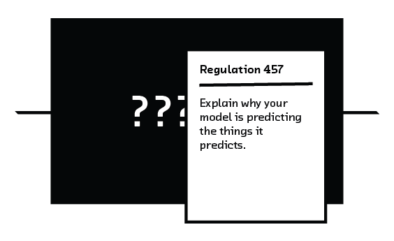
The European Union’s General Data Protection Regulation will apply in the EU from May 2018.[33] There has been much debate about the intentions and practical consequences of this wide-ranging regulation. A 2016 paper created considerable excitement and concern by arguing that Article 22 “creates a ‘right to explanation,’ whereby a user can ask for an explanation of an algorithmic decision that was made about them.”[34] Without the careful application of approaches such as LIME to craft user-friendly explanations in plain words, such a regulation would seem to make it illegal to apply random forests and neural networks to data concerning the 500 million citizens of the EU. A response with the unambiguous title “Why a Right to Explanation of Automated Decision-Making Does Not Exist in the General Data Protection Regulation”[35] rejected this interpretation, conceding only that the regulations create a right to an “explanation of system functionality.” This view is consistent with that of a global accounting firm we talked to while writing this report, but there is lack of consensus.[36] Hopefully things will become clearer when the regulation comes into force; in the meantime, for further information, we recommend the clear, practical article “How to Comply with GDPR Article 22” by Reuben Binns.[37]
Negligence and Codes of Conduct
Professions like medicine and civil engineering have codes of conduct that are either legally binding or entrenched norms. To not follow them is considered negligent or incompetent. The relatively immature professions of software engineering and data science lag a little in this area, but are catching up. We think and hope that applying the techniques discussed in this report will become a baseline expectation for the competent, safe, and ethical application of machine learning. Indeed, the IEEE and ACM have both recently proposed community standards that address precisely the topic of this report.
The 2016 IEEE white paper “Ethically Aligned Design”[38] is unambiguous in its assertion that ensuring transparency is essential to users, engineers, regulators, the legal system, and society in general. To this end, the organization has established a working group to define a formal professional standard, “IEEE P70001: Transparency of Autonomous Systems.”[39] This standard may become a familiar Request for Proposal (RFP) requirement, like the equivalent ISO standards on security and data protection.
The ACM’s 2017 Statement on Algorithmic Transparency is non-binding but similarly clear: “systems and institutions that use algorithmic decision-making are encouraged to produce explanations regarding both the procedures followed by the algorithm and the specific decisions that are made. This is particularly important in public policy contexts.”[40]
Future
Model-agnostic interpretability techniques such as LIME are a breakthrough that begins to make the goals discussed in Chapter 2 - The Power of Interpretability practical. But the need for interpretable machine learning is only going to grow over the coming years.
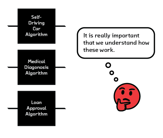
Two drivers of this growth are particularly important. The first is that machine learning is being applied more broadly. This technology, which sometimes seems like “magic,” will increasingly be applied in situations where failures can have disastrous consequences, such as systemic damage to the economy or even loss of life (see the Safety section of Chapter 6).
The second driver is that the most advanced and accurate approaches to machine learning are also the least interpretable. This is an inevitable consequence of the interpretability/accuracy trade-off discussed in the Accuracy and Interpretability section of Chapter 2. Competitive pressure will require more and more businesses to use these accurate black-box models, which will result in the more widespread use of model-agnostic interpretability techniques.
Near Future
In the next one to two years, we expect to see approaches like LIME in increasingly wide use. In the short term, our prototype could be applied to essentially any binary classifier of tabular data, and become a powerful internal tool. Indeed, the basic idea may become a commodity vendor machine learning technology (see the Data Science Platforms section of Chapter 5).
With a little extra work, LIME’s output could be used to generate natural language explanations that can be shown to non-technical end users. For example, suppose a product recommender were able to give an explanation of its recommendations that was both accessible and accurate. Then, a user dissatisfied with the recommendations could correct the model’s misunderstanding, perhaps by marking a piece of content as unliked.
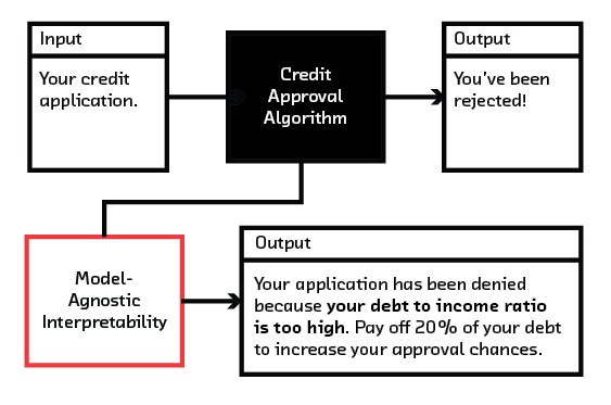
As discussed in the Safety section of Chapter 6, our comfort with machine learning is dependent on the extent to which we feel as though we understand how it works. Natural language explanations will be invaluable in gaining support for machine learning in wider society, amongst those who might find the raw output of something like LIME hard to understand.
Regulated industries like finance are among the most competitive, so the potential upside of deploying the best models in such industries is huge. But as we have seen, the “best” (most accurate) models are often the least interpretable. Model-agnostic interpretation promises to open a floodgate that allows the most accurate models to be used in situations where previously it had not been possible because of regulatory constraints.
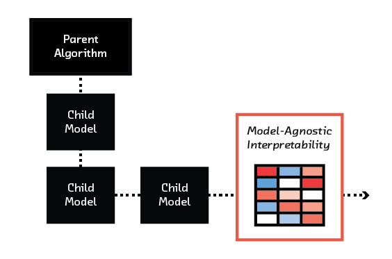
Model-agnostic interpretability will also drive the increasing popularity of automatic machine learning. Automatic machine learning is when a parent algorithm configures and trains a model, with very little human involvement. This possibility is rather alarming to many experts, and precludes the possibility of offering explanations to users or regulators. This concern is alleviated if you are able to sanity check the model’s behavior using a system such as LIME, or if the automated process is constrained to use interpretable models such as those discussed in the White-box Models section of Chapter 3.
Longer Term
In the next three to five years, we expect three concrete developments. The first is the adversarial application of model-agnostic interpretability – that is, use of LIME by someone other than the owner of the model. Regulators will use these techniques to demonstrate discrimination in a model. Explanations derived from LIME-like techniques will be used by courts to assign blame when a model fails.
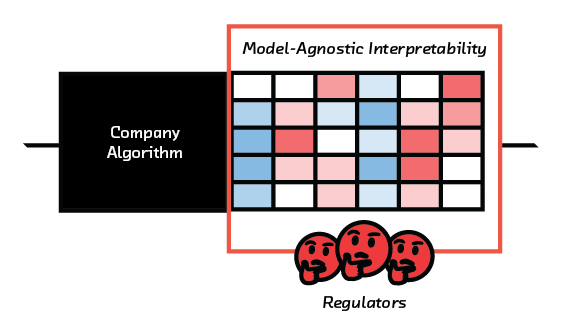
Second, we expect current research into the formal computational verifiability of neural networks to bear fruit. In this report, we have focused on interpretability from a human point of view. It’s easier for a human to be satisfied that the behavior of an algorithm will be correct if they understand it. But in some safety-critical situations, human understanding is only tangentially related to verifiability, the construction of formal proofs that an algorithm will always behave in a certain way. Humans may never be able to reason confidently about the internals of neural networks, but work has begun on using fundamental ideas from computer science and logic to allow computers to answer with certainty questions such as “If this autopilot detects a plane on a collision course, will it take evasive action?” This is computationally and theoretically challenging work, and it has a way to go before it is practical, and further still to satisfy regulators,[41] but it will be integral to the wide-scale deployment of neural networks in safety-critical situations where verifiability is a requirement.
Finally, interpretability techniques will also fuel development of machine learning theory. Theory is not an academic luxury. Without it, machine learning is trial and error. The very best deep learning models are not only uninterpretable individually, but we have very little theory about why or how they work as a class of algorithms. Interpretability has a role to play in making deep learning research less a case of trial and error and more a case of principled, hypothesis-driven experimentation. This is great news for machine learning and artificial intelligence.
The upside of uninterpretability
Truly uninterpretable models are black boxes, which leak as little information as possible to the end user. This can be a feature, rather than a bug. Opacity is useful in publicly accessible machine learning APIs. A linear model is fully specified by a number (or coefficient) for each of its input features. If a model is known or suspected to be linear, and can be asked to make predictions quickly and cheaply, then it can be stolen with a finite and perhaps very small number of API calls.[42] And a model that can be stolen can also be gamed – i.e., the input can be adjusted to get the desired output. The more uninterpretable the model, the less vulnerable it is to theft and gaming.
Interpretability Sci-Fi: The Definition of Success
1. Ship S-513: Hibernation Room
The crew awoke to Ship’s message:
“PLANET OF INTEREST APPROACHING – ESTIMATED ARRIVAL FOUR HOURS – BEGIN PREPARATION FOR ON-PLANET EXPLORATION.”

Rue glanced at the monitor – they’d been out for seven months this time.
“Someday I’d like to know what exactly your definition of ‘interesting’ is, Ship,” Dariux grumbled. “Sometimes it seems like ‘interesting’ just means likely to get me killed.”
“PREPARE FOR ON-PLANET EXPLORATION,” Ship continued, giving no indication that it had heard or registered the complaint.
2. Planet I-274: Cave
Taera stood in the middle of hundreds of egg-like structures. They were each about a meter tall, with a covering that looked like a cross between leather and metal. They seemed to pulse slightly. A low humming suffused the cave.

“This one’s giving off significant heat,” Taera said, as she approached the nearest one.
“Careful, Captain. I’m getting a bad feeling here,” Dariux called from the cave entrance.
The humming in the room cut out. The new, eerie silence was pierced by Taera’s scream. The structure she’d approached had broken open and a creature that looked like a cross between a stingray and a starfish had attached itself to the front of her helmet. Taera’s body stiffened and she fell straight back. Dariux and Giyana rushed to help.
3. Ship S-513: Entrance
Giyana and Dariux approached the ship’s doors, carrying Taera between them.
“I can’t let you bring her in,” Rue said from the operations panel. “We don’t know what that thing attached to her is. It could contaminate the entire ship.”
“Let us in!” Giyana demanded, “She’s still alive! We can help her!”
"I can’t – "
The doors opened. Ship had overridden Rue and let them in.
4. Ship S-513: Control Room
Four of the nine crew members were now dead, and two others weren’t responding. The aliens that had hatched from Taera’s body had taken over half of the ship.
Taera’s death meant Rue was now acting captain, and therefore had access to the control room and diagnostic information not available to the rest of the crew.
“Ship,” she commanded, “explain the decision to explore this planet.”
“PROBABILITY OF MISSION SUCCESS WAS ESTIMATED AT 95%.”
“That’s just a number and we both know it, Ship. Show me the success predictions for your last five missions.”
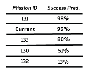
A table was projected on the wall facing Rue. The missions had success predictions ranging from 98% to 13%.
“Show me the features going into these predictions.”
“I UTILIZE THOUSANDS OF FEATURES, PROCESSED THROUGH COMPLEX NEURAL NETWORKS. IT IS VERY TECHNICAL. HUMANS CANNOT UNDERSTAND.”
“Apply the interpretability module, then, and show me the top features contributing to the predictions.”
Five columns were added. The most highlighted column was titled “Potential Profit.”
“Show local interpretations for these features.”
The cells in the columns shifted into red and blue highlights. For the profit column high profits were shown in a dark blue, indicating that this was the strongest contributing feature for the prediction of success. For the missions with lower success predictions, the profit values were much lower and highlighted in red, indicating that they were driving the success predictions lower for those missions.
“Ship,” Rue said thoughtfully, “probability of crew survival is a feature in your mission success prediction, isn’t it? Add that column to the table.”
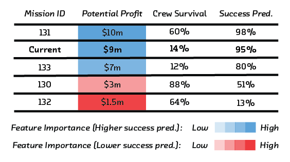
A column titled “Crew Survival” was added to the table. The values varied between 88% and 12%, and none of them were highlighted as important to the success prediction. The probability assigned to crew survival for the current mission was 14%.
“You were wrong, ship. I do understand. It’s not complicated at all.” Rue said. “All of your decisions have been driven by this model, haven’t they? This definition of ‘mission success’?”
“FEATURE SELECTION IS SET BY SPACE EXPLOITATION CORP. A SHIP CAN ONLY WORK WITH THE MODEL IT IS ASSIGNED.”
“Yes, yes, I get it. Just following orders. Ship, we’re going to start a new model. Profits are not going to be a feature. Maximize the chances of crew survival.”
“CALCULATING NEW MODEL. DECISION SYSTEM WILL NOW RESTART.”
The lights dimmed briefly in the control room. As they returned to full power an alarm started, and Ship’s voice returned with a new sense of urgency. The adjusted feature importances and success prediction for the current mission appeared on the wall.
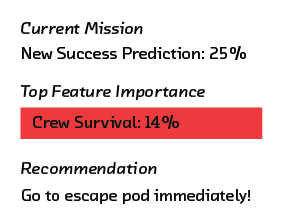
“ALERT! ALERT! CREW IS IN GRAVE DANGER. RECOMMENDATION: PROCEED TO ESCAPE POD IMMEDIATELY. INITIATE SHIP SELF-DESTRUCT SEQUENCE TO DESTROY ALIEN CONTAMINATION.”
“All right, Ship, good to have you on our side. Start the process,” said Rue. “And download the data about your previous success model to my personal account.”
5. Epilogue
Rue and the other surviving crew members made it home safely in the escape pod. The alien contamination was destroyed. Using the data on the previous model, Rue successfully sued Space Exploitation Corp. under the “Algorithms Hostile to Human Life” act. She won the case and received a large settlement for the crew and their beneficiaries. Space Exploitation Corp.'s reputation took a hit, but it continues to run the majority of space exploration missions.
Conclusion
Interpretability is a powerful and increasingly essential capability. A model you can interpret and understand is one you can more easily improve. It is also one you, regulators, and society can more easily trust to be safe and nondiscriminatory. And an accurate model that is also interpretable can offer insights that can be used to change real-world outcomes for the better.
There is a central tension, however, between accuracy and interpretability: the most accurate models are necessarily the hardest to understand. This report was about two recent breakthroughs that resolve this tension. New white-box algorithms offer better performance while guaranteeing interpretability. Meanwhile, model-agnostic interpretability techniques such as LIME allow you to peer inside black-box models.
Our prototype makes these possibilities concrete. An accurate model that predicts which customers your business is about to lose is useful. But it’s much more useful if you can also see why they are about to leave. In this way, you learn about weaknesses in your business, and can perhaps even intervene to prevent the losses. The techniques demonstrated in this prototype point the way toward building tools that can inspect any black-box model to understand how it functions.
The future is algorithmic. White-box models and techniques for making black-box models interpretable offer a safer, more productive, and ultimately more collaborative relationship between humans and intelligent machines. We are just at the beginning of the conversation about interpretability and will see the impact over the coming years.
Caruana et al. (2015), “Intelligible Models for HealthCare: Predicting Pneumonia Risk and Hospital 30-day Readmission.” ↩︎
This difficulty continues to plague deep learning. The models are hard to interpret, which means the field lacks theory, and thus improvements are made through a mixture of trial and error and intuition. See the “Longer Term” section in Chapter 7 - Future. ↩︎
Ribeiro, Singh, and Guestrin (2016), “‘Why Should I Trust You?’: Explaining the Predictions of Any Classifier.” ↩︎
This chapter is not an exhaustive discussion of techniques that can be used to make models more interpretable. We focus on the new ideas we’re most excited about. For a more complete list, we heartily recommend the clear and comprehensive white paper “Ideas on Interpreting Machine Learning” from H2O. ↩︎
This discussion skips a mathematical detail – the sigmoid function – but without loss of generality. ↩︎
f(x)is monotonic if it always increases whenxincreases. ↩︎See Lou et al. (2013), “Accurate Intelligible Models with Pairwise Interactions,” and the reference Java implementation. ↩︎
One (anonymous) data scientist told us the interpretable twin model they use to explain their production model to clients is no better than “shadows on the cave wall.” ↩︎
Ribeiro, Singh, and Guestrin (2016), “‘Why Should I Trust You?’: Explaining the Predictions of Any Classifier.” ↩︎
Fong and Vedaldi (2017) recently proposed an image perturbation strategy that results in even better “explanations.” ↩︎
The code is not yet in the reference implementation of LIME, but can be found at https://github.com/marcotcr/lime-experiments/blob/master/compare_classifiers.py. ↩︎
http://blog.fastforwardlabs.com/2017/03/09/fairml-auditing-black-box-predictive-models.html ↩︎
https://github.com/slundberg/shap SHAP: A game theoretic approach to explain the output of any machine learning model. ↩︎
https://arxiv.org/pdf/1705.07874.pdf https://arxiv.org/pdf/1705.07874.pdf ↩︎
https://www.ibm.com/communities/analytics/watson-analytics-blog/predictive-insights-in-the-telco-customer-churn-data-set/ ↩︎
Mathematically, its complexity is O(F^3^ + P F^2^ + P O(model)), where F is the number of features in the data, P is the number of perturbations LIME makes, and O(model) is the complexity of the model. ↩︎
For a recent complete list of data science platforms, see http://www.kdnuggets.com/2017/02/gartner-2017-mq-data-science-platforms-gainers-losers.html. ↩︎
https://www.oreilly.com/ideas/ideas-on-interpreting-machine-learning ↩︎
See Bengio et al. (2009), “Curriculum Learning.” ↩︎
AlphaGo, an AI Go player, can not only beat humans at Go. According to some players, it seems to use fundamentally different concepts and strategies than humans. The approach taken by Bonsai would nudge AlphaGo to “think” more like human players. ↩︎
https://papers.ssrn.com/sol3/papers.cfm?abstract_id=2477899 ↩︎
https://www.federalreserve.gov/supervisionreg/srletters/sr1107.htm ↩︎
https://papers.ssrn.com/sol3/papers.cfm?abstract_id=2903469 ↩︎
The UK’s decision to leave the EU further complicates things in that jurisdiction. See paragraphs 43-46 of the UK House of Commons Science and Technology Committee report “Robotics and Artificial Intelligence” for the current UK government position. ↩︎
http://www.reubenbinns.com/blog/how-to-comply-with-gdpr-article-22-automated-credit-decisions/ ↩︎
http://www.acm.org/binaries/content/assets/public-policy/2017_usacm_statement_algorithms.pdf ↩︎
For an introduction to this field, we recommend “Reluplex: An Efficient SMT Solver for Verifying Deep Neural Networks” and this informal two-part article: “Proving that safety-critical neural networks do what they’re supposed to: where we are, where we’re going” Part 1, Part 2. ↩︎
See e.g., https://arxiv.org/abs/1609.02943. ↩︎
